Advanced Excel Course

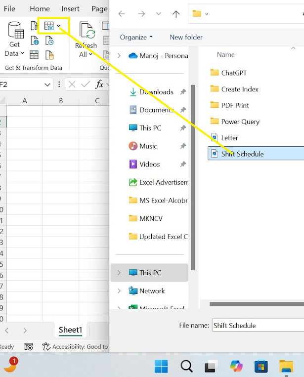
Process Flow to Convert Picture to Text in Office 365 Excel Microsoft Excel in  Office 365  provides a built-in feature to extract text from images using  Insert Data from Picture  and  OneNote OCR . Below is a step-by-step process: 📌 Method 1: Using "Insert Data from Picture" (Directly in Excel) Steps: 1️⃣  Open Excel  in Office 365. 2️⃣ Go to the  "Data"  tab. 3️⃣ Click on  "Get Data" > "From Picture"  > Select  "From File"  or  "From Clipboard"  (if copied). 4️⃣ Select the image containing text. 5️⃣ Excel will process and  convert the image into an editable table . 6️⃣  Review & Edit  the extracted data before inserting it into your sheet. 7️⃣ Click  "Insert" , and the text will appear in the Excel sheet. ✅  Best for:  Tables, structured data, scanned documents. Sample : 🔹 Final Notes For best results, use clear, high-resolution images with proper alignment. OCR accur...

  ✅ Excel Guide: IF and IFS Functions 1️⃣ IF Function 🔍 What is IF? The IF function checks whether a condition is true or false and returns different values based on the result. 📌 Syntax: IF (logical_test, value_if_true, value_if_false) 🧩 Parameters: Argument Description logical_test The condition you want to test (e.g., A1>50) value_if_true The result if the condition is TRUE value_if_false The result if the condition is FALSE 🧾 Example: 🗂️ Data: A (Marks) 85 45 70 🎯 Goal: Label students as "Pass" if marks are ≥ 50, else "Fail" . ✅ Formula: =IF(A2>=50, "Pass", "Fail") 📤 Result: For 85 → Pass For 45 → Fail For 70 → Pass 🪜 Step-by-Step: Click on the cell where you want the result. Type =IF( . Enter the condition (e.g., A2>=50 ). Enter the value for TRUE (e.g., "Pass" ). Enter the value for FALSE (e.g., "Fail" ). Close with a bracket and press Enter . 2️⃣ IFS Fun...

  Process Flow to Sort by Color in Excel  Sorting data by color in Excel allows you to group rows with similar formatting, making it easier to analyze. Follow these steps to sort the data based on the row colors seen in the provided dataset. Step 1: Open Your Excel File Open the Excel file containing your dataset. Ensure the table has colored rows (like blue and gray in your case). Step 2: Select the Data Range Click anywhere inside the table. If needed, manually select the entire data range including column headers (e.g., A1:H5 ). Step 3: Open the Sort Dialog Box Option 1: Using the Data Tab Go to the Data tab on the ribbon. Click on Sort (or press Alt + D + S for shortcut). Option 2: Using the Home Tab Navigate to the Home tab. Click Sort & Filter > Custom Sort . Step 4: Apply Sorting by Color In the Sort window, under the Column section, select the column based on which you want to sort (e.g., SL or Name ). Under Sort On , select Cell Color . Under Order , ...

 Go To Special The "Go To Special" feature in Excel allows users to quickly select specific types of cells, such as blanks, constants, or formulas, for efficient data manipulation. It enhances productivity by streamlining tasks like data cleaning, troubleshooting, and analysis. 1. Blanks Function : Selects all blank cells in the range. Process Flow : Select the range of cells (e.g., A2:D6 ). Navigate to the Home tab, click on Find & Select . Choose Go To Special from the dropdown menu. In the dialog box, select Blanks and click OK . Action : All blank cells in the selected range will be highlighted. Example : Selecting Go To Special > Blanks highlights cells C2, B3, D4, and A5 . Next Step : Fill these blank cells with a value like N/A by typing N/A and pressing Ctrl + Enter . 2. Constants Function : Selects all cells containing constant values (numbers, text, dates). Process Flow : Select the range of cells (e.g., A2:D6 ). Go to Home > Find & Select > ...

Auto Highlight Entire Row & Cell in Excel Objective : Highlight an entire row in Excel based on a condition using VBA. Step 1: Define the Requirement Use Conditional Formatting rule: = CELL("Row")=ROW() Step 2: Write VBA Code (in View Code) Private Sub Worksheet_SelectionChange(ByVal Target As Range) ActiveCell.Calculate End Sub Observe the Result : The entire row corresponding to the selected cell will be highlighted. The row will be highlighted in yellow (or other colors based on your preference). Key Notes: The row will automatically highlight based on the condition. This process works without the need for manual intervention once the macro is run. Process Flow 2: Auto Recalculate Active Cell Objective : Recalculate the formula in the active cell using VBA. Step 1: Write the Conditional Ruling =CELL("address")=CELL("address",A1) Step 2: Process Flow Step 2: Write VBA Code (in View Code) Private Sub Worksheet_SelectionChange(ByVal Target As Range) Ac...

Difference between the DISTINCT and UNIQUE functions: Suppose we have a list of scores: | Name | Score | | --- | --- | | John | 90 | | Mary | 80 | | John | 90 | | David | 70 | | Mary | 80 | | Emma | 95 | We want to analyze the scores using the DISTINCT and UNIQUE functions: DISTINCT Function =DISTINCT(B2:B7) Result: | Score | | --- | | 90 | | 80 | | 70 | | 95 | The DISTINCT function returns all the unique scores. UNIQUE Function =UNIQUE(B2:B7) Result: | Score | | --- | | 70 | | 95 | The UNIQUE function returns only the scores that appear only once. In this example: - The score 90 appears twice, so it's not included in the UNIQUE result. - The score 80 appears twice, so it's not included in the UNIQUE result. - The scores 70 and 95 appear only once, so they're included in the UNIQUE result. This example shows the difference between the DISTINCT and UNIQUE functions: - DISTINCT returns all unique values. - UNIQUE returns only the values that appear only once.