Formula Function
1- Trim
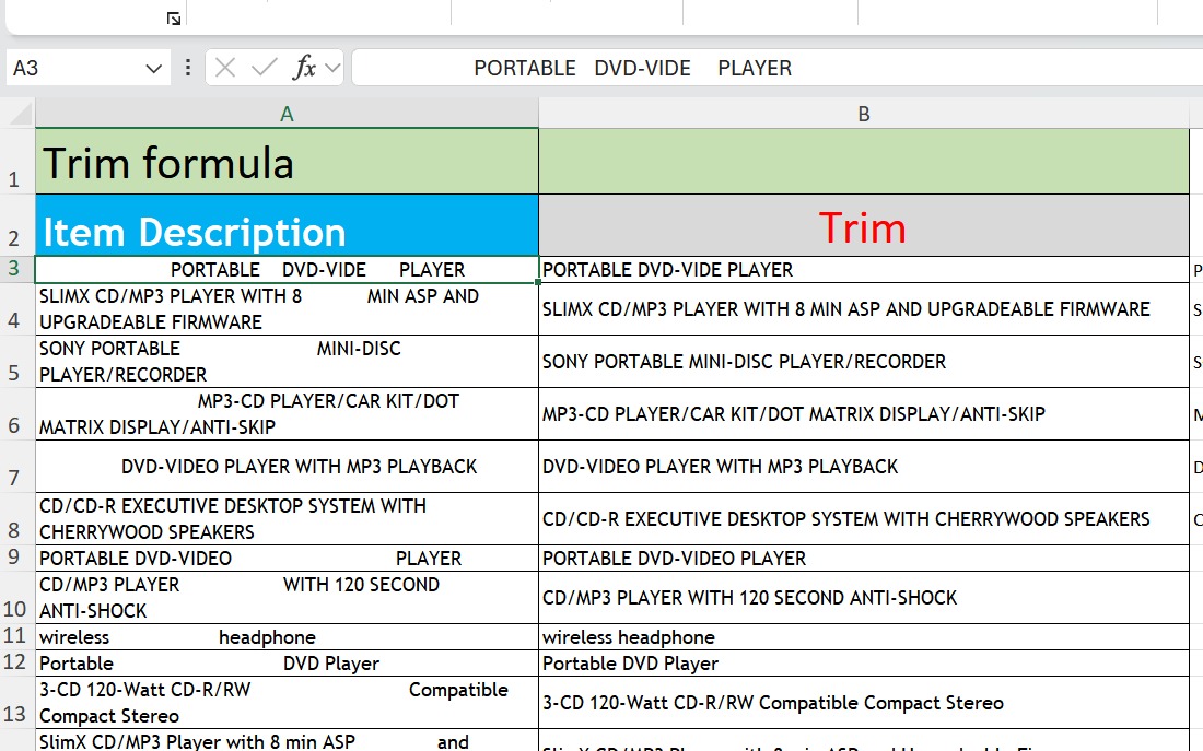
Process Flow to Use the TRIM Function in Excel
1. Open Your Workbook
- Open the Excel file where you want to clean text data.
2. Identify the Data to Trim
- Locate the cell or column containing the text that has extra spaces.
- Example: Column A contains names with irregular spaces.
3. Insert a Helper Column
- Insert a new column next to the text column (if needed).
- Example: Add a column titled "Trimmed Text" next to Column A.
4. Enter the TRIM Formula
- In the first cell of the helper column (e.g., B2), enter the formula: =TRIM(A2)
- Replace
A2with the reference to the cell you want to clean.
5. Apply the Formula
- Drag the fill handle (small square at the bottom-right corner of the selected cell) down to apply the formula to other rows.
6. Replace the Original Data (Optional)
- If you want to replace the original data with the cleaned version:
- Copy the cells with the
TRIMformula. - Right-click on the original column and choose Paste Special > Values.
- Copy the cells with the
7. Verify the Result
- Check the cleaned text for correctness. Extra spaces should be removed.
8. Save Your Work
- Save the workbook to ensure the changes are preserved.
Use Cases
- Clean names: Remove unnecessary spaces in a list of names.
- Prepare data for analysis: Clean text data to avoid errors in lookups or comparisons.
- Standardize text: Ensure consistent spacing in your data.
Let me know if you need additional assistance with Excel formulas! 😊
2- Len
Step-by-Step Process Flow to Use the LEN Function in Excel
Step 1: Open Excel
- Launch Excel and open your desired worksheet.
Step 2: Prepare the Data
- Enter the text or values you want to calculate the length of in the cells.
Step 3: Select the Cell for the Formula
- Click on the cell where you want to display the result of the
LENfunction.
Step 4: Enter the LEN Formula
- In the selected cell, type the formula: =LEN(text)
- Replace
textwith the reference to the cell (e.g.,A1) or the actual text you want to analyze.
Step 5: Execute the Formula
- Press
Enterto calculate the length of the text in the referenced cell.
Step 6: Copy the Formula to Adjacent Cells (Optional)
- Drag the fill handle (small square at the bottom-right corner of the formula cell) down or across to apply the
LENfunction to other cells.
Step 7: Analyze the Results
- The result displayed will show the number of characters in the referenced cell, including spaces and special characters
Sample Picture:

3- Exact Function
Step-by-Step Process Flow to Use the EXACT Function in Excel
Step 1: Open Excel
- Launch Excel and open your desired worksheet.
Step 2: Prepare the Data
- Enter the text values you want to compare in two separate cells.
Step 3: Select the Cell for the Formula
- Click on the cell where you want to display the result of the
EXACTfunction.
Step 4: Enter the EXACT Formula
- In the selected cell, type the formula: =EXACT(text1, text2)
- Replace
text1andtext2with:- The cell references (e.g.,
A1,B1). - Or the actual text strings you want to compare (e.g.,
"Hello","hello").
- The cell references (e.g.,
Step 5: Execute the Formula
- Press
Enterto compare the two texts.- If the texts are identical (case-sensitive), the function will return
TRUE. - If the texts are different, the function will return
FALSE.
- If the texts are identical (case-sensitive), the function will return
Step 6: Copy the Formula to Adjacent Cells (Optional)
- Use the fill handle (small square at the bottom-right corner of the formula cell) to drag and apply the
EXACTfunction to other cells for multiple comparisons.
Step 7: Analyze the Results
- The result will either be
TRUE(if the texts are exactly the same) orFALSE(if they are different).

4- Text Function:
Step-by-Step Process Flow to Use the TEXT Function in Excel
Step 1: Open Excel
- Launch Excel and open your desired worksheet.
Step 2: Prepare the Data
- Enter the date in cell
A1. For example,08-Jan-25.
Step 3: Select the Cell for the Formula
- Click on the cell where you want to display the result of the
TEXTfunction.
Step 4: Enter the TEXT Formula
In the selected cell, type the
TEXTfunction as follows:To display the full day name: =TEXT(A1,"dddd") This will return
Sunday.To display the abbreviated day name: =TEXT(A1,"ddd") This will return
Sun.To display the day as a two-digit number: =TEXT(A1,"dd") This will return
08.To display the day as a single-digit number (without leading zeros): =TEXT(A1,"d")
This will return
8.
Step 5: Execute the Formula
- Press
Enterafter entering each formula to display the corresponding result.
Step 6: Copy the Formula to Adjacent Cells (Optional)
- If needed, use the fill handle (small square at the bottom-right corner of the formula cell) to drag the formula to adjacent cells.
Step 7: Analyze the Results
- The result will vary based on the format you use in the
TEXTfunction: ddddreturns the full day name (e.g.,Sunday).dddreturns the abbreviated day name (e.g.,Sun).ddreturns the day as a two-digit number (e.g.,08).dreturns the day as a single-digit number without leading zeros (e.g.,8).
Sample Picture:

5- INT Function
Step-by-Step Process Flow to Use the INT Function in Excel
Step 1: Open Excel
- Launch Excel and open your desired worksheet.
Step 2: Prepare the Data
- Enter the number or cell reference that you want to round down to the nearest integer.
- Example: Enter
12.75in cellA1.
Step 3: Select the Cell for the Formula
- Click on the cell where you want to display the result of the
INTfunction.
Step 4: Enter the INT Formula
- In the selected cell, type the following formula: =INT(number)
- Replace
numberwith:- The reference to the cell containing the number (e.g.,
A1). - Or the actual number itself (e.g.,
12.75).
- The reference to the cell containing the number (e.g.,
Step 5: Execute the Formula
- Press
Enterto round the number down to the nearest integer.- Example: For
=INT(A1)whereA1contains12.75, the result will be12.
- Example: For
Step 6: Copy the Formula to Adjacent Cells (Optional)
- If you want to apply the
INTfunction to multiple numbers, use the fill handle (small square at the bottom-right corner of the formula cell) to drag the formula down or across.
Step 7: Analyze the Results
- The result will display the largest integer that is less than or equal to the given number, essentially rounding down the value.
- Example:
=INT(12.75)→12=INT(-12.75)→-13
Sample Picture:
